Welcome back, image explorers! Today's voyage leads us to Day 8, where we'll delve into the intriguing realm of image statistics and texture analysis. Inspired by the captivating visual tapestry of Wonder Egg Priority, we'll extract valuable insights about average mean, contrast, and homogeneity to gain a deeper understanding of the image's characteristics. Buckle up and prepare to unlock hidden dimensions within your own visuals!

Technical Gems at our Disposal:

• Grayscale Conversion: cv2.cvtColor() transforms a color image into a single-channel representation, capturing intensity variations.

• Color Channel Splitting: cv2.split() separates an RGB image into its individual red, green, and blue channels for independent analysis.

• Array Flattening: img1.flatten() converts a 2D image array into a 1D vector, enabling statistical calculations like mean and kurtosis.

• Gray-Level Co-occurrence Matrix (GLCM): This texture analysis tool greycomatrix() reveals how pairs of pixels with specific intensity values are distributed within an image, providing valuable insights into its spatial patterns.

• GLCM Properties (greyprops): greycoprops() extracts quantitative texture measures like contrast, homogeneity, and energy from the GLCM, quantifying aspects like sharpness and smoothness.

Unveiling Wonder Egg Priority's Secrets:

1. Mean Intensity: We'll calculate the average mean (np.mean()) of the entire grayscale image and individual color channels, providing a basic understanding of overall brightness and color balance.

2. Kurtosis: This statistical measure (kurtosis()) reveals the "tailedness" of the image's intensity distribution, indicating the presence of extreme intensity values (bright highlights or dark shadows).

3. GLCM Texture Analysis: We'll construct a GLCM using greycomatrix() and then extract key texture features like contrast and homogeneity using greycoprops().

1. Import Libraries

from skimage.util import img_as_ubyte
import cv2 
import numpy as np
import matplotlib.pyplot as plt
from skimage import io
from pylab import *

The main package of skimage only provides a few utilities for converting between image data types; for most features.

\****New Package\***

img_as_ubyte : Convert an image to unsigned byte format, with values in [0, 255].

2. Loading and Splitting Channels:

• Load the image:

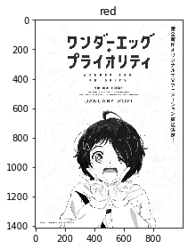
    img = cv2.imread('../input/wondereggpriority/Wonder_Egg_Priority_Key_Visual.png')
  

  • cv2.imread(): Loads the image from the specified path. Remember to update the path if needed.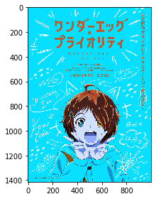

    

• Convert to grayscale:

    img1 = cv2.cvtColor(img, cv2.COLOR_BGR2GRAY)
  

  • cv2.cvtColor(): Converts the color image to grayscale, discarding color information.

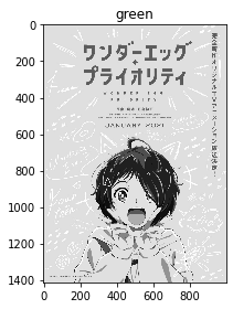
• Split into color channels:

    blue, green, red = cv2.split(img)
    figure(0)
    title("blue")
    io.imshow(blue)
    figure(1)
    title("green")
    io.imshow(green)
    figure(2)
    title("red")
    io.imshow(red)
  

  cv2.split(): Splits the original color image into its three individual Blue, Green, and Red channels, allowing analysis of each color component separately.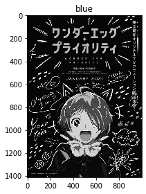

  

  

  

3. Calculating Average Mean:

• Grayscale image:

    Avg_mean_gray = np.mean(img1)
    print("Avg_mean_gray: " + str(Avg_mean_gray))
  

  • np.mean(): Calculates the average value (intensity) of all pixels in the specified array.

• Individual color channels:

    Avg_mean_blue_channel = np.mean(blue)
    Avg_mean_green_channel = np.mean(green)
    Avg_mean_red_channel = np.mean(red)
    print("Avg_mean_blue_channel: " + str(Avg_mean_blue_channel))
    print("Avg_mean_green_channel: " + str(Avg_mean_green_channel))
    print("Avg_mean_red_channel: " + str(Avg_mean_red_channel))
  

  • Here, we calculate the mean for the entire grayscale image (img1) and for each individual color channel (blue, green, red).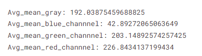

    

4. Exploring Kurtosis:

• Flatten the grayscale image:

    img_flat = img1.flatten()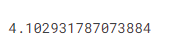
  

  

  • img1.flatten(): Converts the 2D grayscale image array into a 1D vector, making it suitable for statistical calculations.

• Calculate kurtosis (measure of "tailedness"):

    from scipy.stats import norm, kurtosis
    kurtosis(img_flat)
  

  • scipy.stats.kurtosis(): Calculates the kurtosis of the pixel intensity distribution, indicating how "peaked" or "tailed" it is.

  • Higher kurtosis suggests the presence of more extreme intensity values (bright highlights or dark shadows), while lower kurtosis indicates a more uniform distribution.

5. Calculating GLCM Features:

• Convert to grayscale (again) and quantize:

    gray = color.rgb2gray(img)
    image = img_as_ubyte(gray)
    bins = np.array([0, 16, 32, ..., 240, 255])
    inds = np.digitize(image, bins)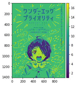
  

  

  • color.rgb2gray(): Converts the color image to grayscale again, even though it was already done in step 1. This seems unnecessary in this context.

  • bins: Defines an array of intensity values that will be used to create bins for pixel quantization.

  • np.digitize(): Assigns each pixel a bin index based on its intensity value, essentially grouping pixels with similar intensities.

  • img_as_ubyte(): Ensures image data type is appropriate for the np.digitize() function.

• Create GLCM (Gray-Level Co-occurrence Matrix):

    GLCM_Matrix = greycomatrix(inds, [1], [0, np.pi/4, np.pi/2, 3*np.pi/4])
  

  

  • greycomatrix(): Creates a Gray-Level Co-occurrence Matrix (GLCM) based on the binned image data.

    • distance=1: Considers pixel pairs with a horizontal distance of 1 pixel.

    • angles=[0, np.pi/4, np.pi/2, 3*np.pi/4]: Calculates GLCM for four different directions (0°, 45°, 90°, 135°).

6. GLCM (2nd Order)

#GLCM features (2nd order)
fig = plt.figure(figsize=(15, 10))

1. Creating the Figure:

• fig = plt.figure(figsize=(15, 10)): This line creates a figure object with a specific size (15 and 10 units). This essentially defines the canvas on which your visualization will be displayed.

contrast = greycoprops(GLCM_Matrix, 'contrast')
dissimilarity = greycoprops(GLCM_Matrix, 'dissimilarity')
homogeneity = greycoprops(GLCM_Matrix, 'homogeneity')
energy = greycoprops(GLCM_Matrix, 'energy')
correlation = greycoprops(GLCM_Matrix, 'correlation')

2. Loading Extracted Features:

• Each line (contrast = ..., dissimilarity = ..., etc.) assumes you have already calculated different texture features (contrast, dissimilarity, homogeneity, energy, and correlation) from the GLCM matrix. These lines simply assign the calculated values to corr

  esponding variables for further use.

3. Creating Subplots for Visualization:

fig.add_subplot(3, 3, 1)

• fig.add_subplot(3, 3, 1) and similar lines create individual subplots within the figure. The numbers 3 and 3 specify a 3x3 grid arrangement, and the final number (e.g., 1) indicates the position within the grid (top-left being 1). Each feature will be displayed on its own subplot.

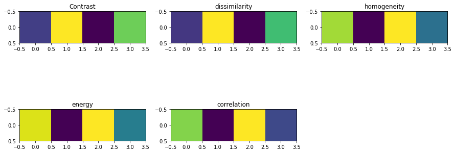
4. Visualizing Each Feature:

plt.imshow(contrast)
plt.axis()
plt.title("Contrast")
fig.add_subplot(3, 3, 2)
plt.imshow(dissimilarity)
plt.axis()
plt.title("dissimilarity")
fig.add_subplot(3, 3, 3)                
plt.imshow(homogeneity)
plt.axis()
plt.title("homogeneity")
fig.add_subplot(3, 3, 4) 
plt.imshow(energy)
plt.axis()
plt.title("energy")
fig.add_subplot(3, 3, 5) 
plt.imshow(correlation)
plt.axis()
plt.title("correlation")

• Within each subplot:

  • plt.imshow(feature): This line displays the feature (represented by the variable, e.g., contrast) as an image on the corresponding subplot. This essentially converts the numerical values into a visual representation.

  • plt.axis(): This line removes the axis ticks and labels from the subplot, providing a cleaner visualization focused on the image itself.

  • plt.title("Feature Name"): This line sets the title of the subplot to the corresponding feature name (e.g., "Contrast"), making it clear what each image represents.

Beyond Wonder Egg Priority:

Remember, these techniques are adaptable! Apply them to your own images to:

• Compare and contrast visual styles.

• Understand how image processing techniques affect overall appearance.

• Develop tools for automated image classification or analysis.

Ready to Dive Deeper?

Join the discussion and share your insights! Ask questions, present your own image explorations, and